Introduction
Value Numbering is a universally useful optimization implemented by most compilers like Clang, GCC, etc. Traditionally GVN can be divided into Hash-Based and Value-Partitioning. The former handles algebraic simplifications but locally. The latter is global but handling only simple redundancies. K. C and T. S came up with a new method to solve it for SSA.
SCC-Based Value Numebring (Easy Version)
This paper proposed an \(O(N \cdot D(SSA))\) algorithm at first, which is based on the RPO traversal and SSA form IR.
Note: RPO traversal guarantees that predecessors through non-back edges of BasicBlocks are processed before the block itself
Here is pseudocode for this easy version:
1 | VN.fill(Null) |
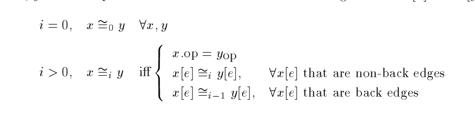
We define equivalence/congruence relation, \(\cong_i\). We say that \(x \cong_i y\) if and only if \(VN[x] = VN[y]\) after \(i^{th}\) RPO iteration.
We get:
Now we prove the correctness.
Firstly, it's obvious that \(x \cong_i y \rightarrow x \cong_{i-1} y\). It's monotonicity.
And each step produces a re nement of the partition, and refinement cannot continue indefinitely. Since the RPO algorithm begins with all SSA names congruent, we must converge to the same fixed point as value partitioning.
Then, we try to get its time complexity. Back edges play a key role here.
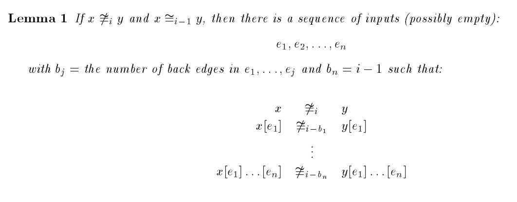
Induction for \(x \ncong_{i} y\):
Basis (\(i = 1\)): Empty sequence
Basics (\(j=1\)) and Induction: (\(i > 1\)):
- case1: \(x.op \ne y.op\). Obviously impossible due to \(x \cong_{i-1} y\).
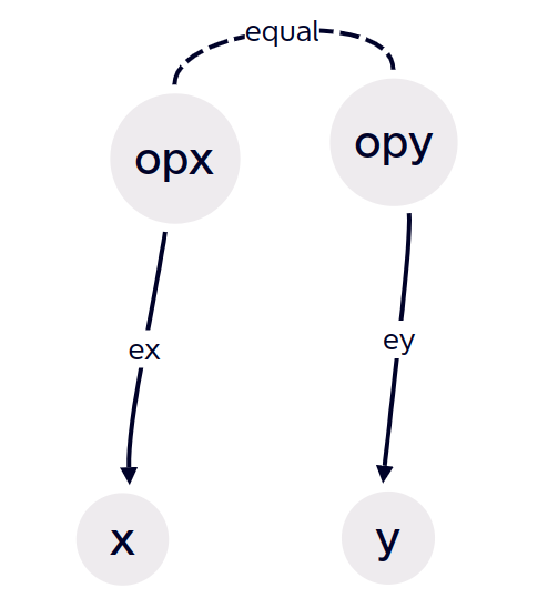
- case2: \(x[e_1] \ncong_{i} y[e_1]\) for some non-back edge. Some here means that there exists non-back edge \(e\) cause it. But that contradicts with \(x \cong_{i - 1} y\). Just like graph below, it's impossible:
- case 3: \(x[e_1] \ncong_{i-1} y[e_1]\) for some back edge. That's possible. Sequence now consists of \(e\).
Induction (\(j > 1\))
case1: \(x.op \ne y.op\). Obviously impossible as before.
case2: \(x[e_j] \ncong_{i} y[e_j]\) for some non-back edge. The sequence consists of \(e\) followed by the sequence for the pair \(x[e_{j-1}],y[e_{j-1}]\), which we know exists by the induction hypothesis for \(j\): \(s\)
case 3: \(x[e_j] \ncong_{i-1} y[e_j]\) for some back edge. The sequence consists of \(e_j\) followed by the sequence for the pair \(x[e],y[e]\), which we know exists by the induction hypothesis for \(i\).
Final time analysis (\(D(SSA)\) is the loop connectedness): 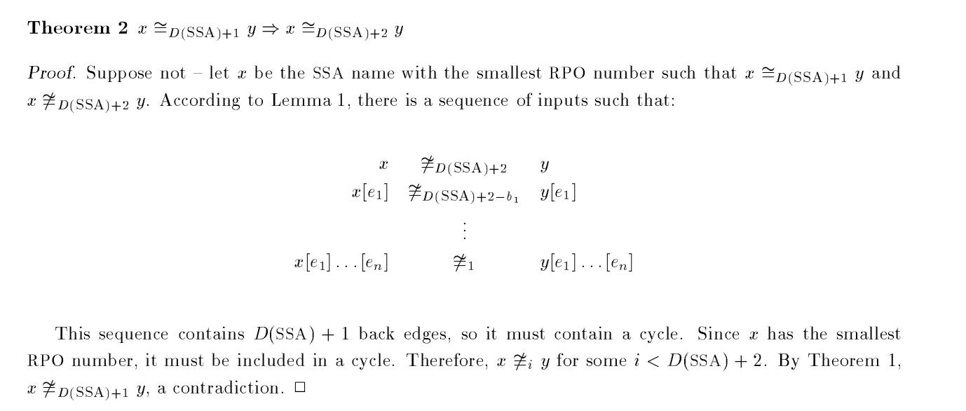
The SCC Algorithm (More efficient)
To make the algorithm more efficient in practice, we operate on the SSA graph instead of the control-flow graph. We refer to the improved algorithm as the SCC algorithm because it concentrates on the strongly connected components of the SSA graph.
The paper works with Tarjan's depth-first algorithm for finding SCCs. Just handle the single node firstly and then handle nodes in SCCs in RPO order.
Result
Not worse than Hash-Based and Value-Partitioning methods. Details in paper.
Connection with modern compilers
NewGVN in LLVM applies the algorithm in this paper, in development still.
Reference
- SCC-Based Value Numbering, by Keith Cooper and Taylor Simpson