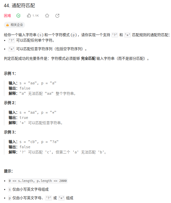
0%

题目描述: img

动态规划

简单想法:

使用动态规划,令 \(dp[i][j]\)是否 \(s[0..i]\)\(p[0..j]\) 匹配 ,也就是 s 前 i 个字符与 p 前 j 个字符匹配。

则有初始状态:

\[dp[0][0] = true\]

由于长度大于 0 的字符串不可能被长度为 0 的模式匹配,故令:

\[dp[i][0] = false, 0 < i \le sn\]

同时长度为 0 的字符串只可能被形如"*"这样全为通配符的模式匹配,故令:

\[dp[0][j] = dp[0][j-1] \quad \wedge \quad p[j-1] = '*'\]

状态转移方程则为:

\[ \begin{equation*} %加*表示不对公式编号 \begin{split} dp[i][j] = & dp[i][j - 1] \wedge p[j - 1] = '*' \quad \vee \\ & dp[i - 1][j] \wedge p[j - 1] = '*' \quad \vee \\ & dp[i - 1][j - 1] \wedge (s[i - 1] = p[j - 1] \vee p[j - 1] = '?' \vee p[j - 1] = '*') \end{split} \end{equation*} \]

故我们可以有代码:

1
2
3
4
5
6
7
8
9
10
11
12
13
14
15
16
17
18
19
20
21
22
23
24
25
26
27
28
29
30
31
32
33
34
bool dp[2001][2001];

class Solution {
public:
bool isMatch(string s, string p) {
if (s.length() == 0 &&
std::all_of(p.begin(), p.end(), [](char c) { return c == '*'; }))
return true;
if (p.length() == 0)
return false;

int sn = s.length();
int pn = p.length();
dp[0][0] = 1;
for (int i = 1; i <= pn; ++i) {
dp[0][i] = std::all_of(p.begin(), p.begin() + i,
[](char c) { return c == '*'; });
}
for (int i = 1; i <= sn; ++i) {
dp[i][0] = false;
}
for (int i = 1; i <= sn; ++i) {
for (int j = 1; j <= pn; ++j) {

bool a = dp[i][j] =
(dp[i][j - 1] && p[j - 1] == '*') ||
(dp[i - 1][j] && p[j - 1] == '*') ||
(dp[i - 1][j - 1] &&
(s[i - 1] == p[j - 1] || p[j - 1] == '?' || p[j - 1] == '*'));
}
}
return dp[sn][pn];
}
};

时间复杂度为 \(O(mn)\), 空间复杂度为 \(O(mn)\)

贪心(LeetCode 题解)

前一方法的瓶颈在于对星号 \(*\) 的处理方式:使用动态规划枚举所有的情况。由于星号是「万能」的匹配字符,连续的多个星号和单个星号实际上是等价的,那么不连续的多个星号呢?

我们以 \(p=∗ abcd ∗\) 为例,ppp 可以匹配所有包含子串 abcd 的字符串,也就是说,我们只需要暴力地枚举字符串 s 中的每个位置作为起始位置,并判断对应的子串是否为 abcd 即可。这种暴力方法的时间复杂度为 O(mn),与动态规划一致,但不需要额外的空间。

如果 p=∗abcd∗efgh∗i∗ 呢?显然,ppp 可以匹配所有依次出现子串 abcd、efgh、i 的字符串。此时,对于任意一个字符串 sss,我们首先暴力找到最早出现的 abcd,随后从下一个位置开始暴力找到最早出现的 efgh,最后找出 i,就可以判断 sss 是否可以与 ppp 匹配。这样「贪心地」找到最早出现的子串是比较直观的,因为如果 sss 中多次出现了某个子串,那么我们选择最早出现的位置,可以使得后续子串能被找到的机会更大。

因此,如果模式 ppp 的形式为 \[* u_1 * u_2 * u_3 * \cdots * u_x ∗\] ,即字符串(可以为空)和星号交替出现,并且首尾字符均为星号,那么我们就可以设计出下面这个基于贪心的暴力匹配算法。算法的本质是:如果在字符串 sss 中首先找到 \(u_1\) ,再找到 \(u_2, u_3, \cdots, u_x\),那么 s 就可以与模式 p 匹配,伪代码如下:

1
2
3
4
5
6
7
8
9
10
11
12
13
14
15
16
17
18
19
20
21
22
23
24
25
26
27
28
29
30
31
32
33
34
35
36
37
38
// 我们用 sIndex 和 pIndex 表示当前遍历到 s 和 p 的位置
// 此时我们正在 s 中寻找某个 u_i
// 其在 s 和 p 中的起始位置为 sRecord 和 pRecord

// sIndex 和 sRecord 的初始值为 0
// 即我们从字符串 s 的首位开始匹配
sIndex = sRecord = 0

// pIndex 和 pRecord 的初始值为 1
// 这是因为模式 p 的首位是星号,那么 u_1 的起始位置为 1
pIndex = pRecord = 1

while sIndex < s.length and pIndex < p.length do
if p[pIndex] == '*' then
// 如果遇到星号,说明找到了 u_i,开始寻找 u_i+1
pIndex += 1
// 记录下起始位置
sRecord = sIndex
pRecord = pIndex
else if match(s[sIndex], p[pIndex]) then
// 如果两个字符可以匹配,就继续寻找 u_i 的下一个字符
sIndex += 1
pIndex += 1
else if sRecord + 1 < s.length then
// 如果两个字符不匹配,那么需要重新寻找 u_i
// 枚举下一个 s 中的起始位置
sRecord += 1
sIndex = sRecord
pIndex = pRecord
else
// 如果不匹配并且下一个起始位置不存在,那么匹配失败
return False
end if
end while

// 由于 p 的最后一个字符是星号,那么 s 未匹配完,那么没有关系
// 但如果 p 没有匹配完,那么 p 剩余的字符必须都是星号
return all(p[pIndex] ~ p[p.length - 1] == '*')

当然还有一些特殊情况,如星号不总是出现在前后,此处省略。 时间复杂度: 渐进:\(O(mn)\),平均复杂度:\(O(m\log{n})\) 具体的分析可以参考论文On the Average-case Complexity of Pattern Matching with Wildcards,注意论文中的分析是对于每一个\(u_i\) 而言的,即模式中只包含小写字母和问号,本题相当于多个连续模式的情况。由于超出了面试难度。这里不再赘述。

空间复杂度:O(1)

此外(LeetCode 官方题解)

在贪心方法中,对于每一个被星号分隔的、只包含小写字符和问号的子模式 \(u_i\) ,我们在原串中使用的是暴力匹配的方法。然而这里是可以继续进行优化的,即使用 AC 自动机 代替暴力方法进行匹配。 由于 AC 自动机本身已经是竞赛难度的知识点,而本题还需要在 AC 自动机中额外存储一些内容才能完成匹配,因此这种做法远远超过了面试难度。 这里只给出参考讲义 Set Matching and Aho-Corasick Algorithm

  • 讲义的前 6 页介绍了字典树 Trie;

  • 讲义的 7−19 页介绍了 AC 自动机,它是以字典树为基础的;

  • 讲义的 20−23 页介绍了基于 AC 自动机的一种 wildcard matching 算法,其中的 wildcard \(\phi\) 就是本题中的问号。

感兴趣的读者可以尝试进行学习。

Making routing scalable

Here are some concepts to note:

scale: billions of destinations:

  • can't store all destinations in routing tables.
  • routing table exchange would swamp links.

administrative autonomy:

  • Internet: a network of networks
  • each network admin may want to control routing in its own network

Approach to scalable routing

We always aggregate routers into regions known as "autonomous systems" (a.k.a "domains").

And intra-AS (intra-domain) is such routing among routers within same AS(network).

  • all routers in AS must run same intra-domain protocol.
  • routers in different AS can run different intra-domain protocols.
  • gateway router: at edge of its own AS, has link(s) to router(s) in other AS'es

inter-AS routing among AS'es is the gateways perform inter-domain routing

Both of them determine entries for destination of routers, while former is within AS and latter is for external destinations. Most common intra-AS routing protocols:

  • RIP (Routing Information Protocol), which is no longer widely used.
  • OSPF (Open Shortest Path First), which includes classic link-state routing.
  • EIGRP: (Enhanced Interior Gateway Routing Protocol), which is DV based/

OSPF

OSPF is an intra-domain routing protocol.

  • open: publicly available

  • classic link-state:

    • each router floods OSPF link-state advertisements (directly over IP) to all other routers in entire AS.
    • multiple link costs metrics possible: bandwidth, delay.
    • global (has full topology)

    There is two-level hierarchy: local area and backbone.

    • Local routers only know/compute detailed topology within its local area, and forwad information to area border routers.
    • And area border routers are responsible for summarizing distances to destinations in own area, and advertising in backbone.

BGP

BGP is an inter-domain routing protocol ("glue that holds the Internet together").

BGP provides each AS a means to:

  • obtain destination network reachability information from neighboring ASes (eBGP).
  • determine roues to other networks based on reachability information and policy.
  • propagate reachability information to all AS-internal routers (iBGP).
  • advertise destination reachability information.

BGP Basics

BGP Session: two BGP routers exchange BGP messages over semi-permanent TCP connection:

  • advertising paths to different destination network prefixes
  • BGP is a "path vector" protocol

BGP protocol messages [RFC 4371]:

  • Open: opens TCP connection to peer and authenticates sending BGP peer
  • Update: advertises new path (or withdraws old)
  • Keepalive: keeps connection alive in absence of UPDATES; also ACKS OPEN request
  • Notification: reports erros in previous msg; also used to close connection

BGP: path advertisement

BGP advertised path: prefix + attributes

  • path prefix: destination being advertised
  • two important attributes:
    • AS-PATH: list of ASes through which prefix advertisement has passed
    • NEXT-HOP: indicates specific internal-AS router to next-hop AS

BGP policy

ISP only wants to route traffic to/from its customer networks (does not want to carry transit traffic between other ISPs – a typical “real world” policy)

BGP: populating forwading tables

Just popluate from boundary to internal and choose local gateway that has least intra-domain cost. Omit details here.

Benefits

Intra/Inter-AS routing scale the network, creating hierarchical routing, reducing forwarding table size. And seperate them can make:

  • intra-AS focus on performance.
  • inter-AS has policy dominates over performaance.

Routing algorithm goal: determine good paths from sending hosts to receiving host. So what is a good path? Here "good" means least cost, fastest and least congested. Cost is defined by network operator: related to bandwidth, related to congestion, etc.

For the characterisitics of network, We apply graph abstraction to solve this problem. Let routers be vertices, connections be edges and the "cost" of connection be weights of edges.

There is routing algorithm classification:

  • global: all routers have complete topology, link cost info
  • decentralized: iterative process of computation, exchange of info with neighbors
  • dynamic: routes change more quickly
  • static: routes change slowly over time

Link State Algorithm is iterative and centralized/global, which knows network topology, link costs needed. And it computes least cost paths from one node to all other nodes.

Notation: \(C_{a,b}\) is the cost from \(a\) to \(b\). \(D(a)\) is the cost of least-cost-path from source to destination \(a\). \(p(a)\) is the predecessor node along path from source to \(a\). And \(N'\) is set of nodes whose least-cost-path definitively known.

And it's mostly the same as Dijkstra's Algorithm or Prim Algorithm in Graph Theory. Omit details here.

Optimized algorithm complexity: \(O(nlogn)\)

Message Complexity: Each router must broadcast its link state information to other \(n\) routers, so complexity is \(O(n^2)\)

Distance Vector

Distance Vector is an application of Bellman Ford Algorithm, which is decentralized, iterative and asynchronous. In this algorithm, each node propagates its cost(distance vector) to its neighbors, so that they can update their own distance vectors.

The process for each node is: - wait for change in local link cost or msg from neighbor - recompute its own DV estimates with DV received from neighbor - if its own DV changed, send it to its neightbors

Such thing is like state information diffusion. As a compiler learner, I think it's the same as what MFP(Maximum FixedPoint) implements

However, there's difference where one of the costs increase. For example, with path x-4-y-1-z, when \(C_{x,y}\) updates to 60, \(y\) will update \(D_y(x)\) to 6 because \[D_y(x) = min(D_y(x), C_{y,z} + D_z(x))\], while \(D_z(x)\) is out-of-date. Such count-to-infinity problem is tricky to solve.

Message complexity: exchange between neighbors; convergence time varies.

Comparsion of LS and DV algorithms

robustness: - LS: - router can advertise incorrect link cost. - each router computes only its own table.

  • DV:
    • DV router can advertise incorrect path cost:black-holing.
    • each router;s DV is used by others: error propagate through network.

Classic TCP

AIMD

AIMD - a distributed, asynchronous algorithm - has been shown to:

  • optimize congested flow rates network wide.
  • have desirable stability properties.

Approach: senders can increase sending rate until packet loss occurs, then decrease sending rate on loss event.

Additive Increase: Increase sending rate by 1 maximum segment size every RTT until loss detected.

Multiplicative Decrease: Cut sending rate in half at each loss event by triple duplicate ACK (TCP Reno). Or cut to 1 maximum segment size when loss is detected by timeout (TCP Tahoe)

TCP Congestion Control Details

sender sequence number space:

/images/SenderSequenceSpace.png

TCP rate ~= \(\frac{cwnd}{RTT}\) bytes/sec

  • TCP sender limits transmission : LastByteSent - LastByteAcked <= cwnd
  • cwnd is dynamically adjusted in response to observed network congestion

TCP slow start

initially cwnd = 1 MSS. double cwnd every RTT. done by incrementing cwnd for every ACK received.

When cwnd gets to 1/2 of its value before, we should switch to linear

CUBIC

CUBIC

TCP CUBIC is default in Linux, most popular TCP for popular Web servers.

Enhanced TCPs

Delay-based TCP congestion control

"Just full enough, but not fuller": keep bottleneck link busy transmitting, but avoid high delays/buffering

Explicit congestion notification (ECN)

TCP deployments often implement network-assisted congestion control.

  • two bits in IP header (ToS field) marked by network router to indicate congestion
    • policy to determine marking chosen by network operator
  • congestion indication carried to destination
  • destination sets ECE bit on ACK segment to notify sender of congestion
  • involves both IP (IP header ECN bit marking) and TCP (TCP header C,E bit marking)

TCP fairness

Goal: Multiple TCP sessions share the equal resource of network.

However, there is no Internet police policing use of congestion control.

DMA serves asa real solution for I/O problems.

  • Device controller transfers data directly to/from memory without involving the processor.
  • Only interrupts once per page (large) once transfer is complete.

The incoming procedure:

  • Receive interrupt from device
  • CPU takes interrupt, begins transfer (instructs DMA to place data at certain address)
  • Device/DMA engine handle the transfer (CPU is free to execute other things)
  • Upon completion, Device/DMA engine interrupt the CPU again

The outgoing procedure:

  • CPU decides to initiate transfer, confirms that external device is ready.
  • CPU takes interrupt, begins transfer (instructs DMA to place data at certain address)
  • Device/DMA engine handle the transfer (CPU is free to execute other things)
  • Device/DMA engine interrupt the CPU again to signal completion

Cache-coherency

DMA writes to memory, leading to incoherency with cache. Here we can see DMA as another processor core, whose coherency has been solved by most modern multiprocessors.

DMA and CPU Sharing Memory

Cycle Stealing mode

  • DMA Engine transfers a byte, releases control, then repeats

Transparent Mode (Maybe best)

  • DMA transfer only occurs when CPU is not using the system bus

Address Translation

Assuming the virtual memory has 1024B, a page has 256B, then the index of page should be: \[\log_2{\frac{1024}{256}} = 2 bit\] So for an 32-bit address, the first 2 bits is the index, while the remaining 30 bits serve as offset.

Page Table

Consist of: [Valid] [Access Rights] [VPN] [PPN]

Valid bit determines whether this virtual page is mapped to a physical page. The mapping VPN to PPN is by looking up the table. The offset from virtual to physical is invariant.

Page Tables are always saved in main memory. And we always create hierarchical page table since page tables is too big. pagetable

Problems

2+ Physical memory accesses per data access is too slow. Since locality in pages of data, there must be locality in the translations of those pages, we could build a separate cache for the page table.

For historical reasons, cache is called a Translation Lookaside Buffer (TLB)

VPN -> TLB -> PPN -> Data (Access Page Table in main memory if messed)

Performance Analysis

VM Performance

Similar to cache. But here, though the rate of page miss is much smaller, page miss will lead to much slower performance. Page fault(Loading page from disk) requires about 20,000,000 cycles, which is destructive. The corresponding miss rate must be quite small to match it.

The 1st period: the CPU executes instructions from some start address (stored in Flash ROM)

  1. BIOS: FInd a storage device and load first sector.
  2. Bootloader: Load the OS kernel from disk into a location in memory and jump into it.
  3. OS Boot: Initialize services, drivers, etc.

Some Concepts

AMAT: Average memory access time. \(AMAT = t_{hit} + rate_{missed} * penalty_{missed}\)

Cache Miss

Sources of Cache Misses:

  • Compulsory: (Like cold start, process migration, 1st reference)
  • Capacity
  • Conflict (Collison)

The Design Solutions:

  • Compulsory:
    • Increase block size
  • Capacity:
    • Increase cache size
  • Conflict:
    • Increase associativity (may increase hit-time)

Miss Penalty

Factors:

  • How big is your memory architecture
  • How big is your block size

Multiple Cache Levels

To minimize AMAT, we need to adjust the type/parameters of cache. But it's hard to reduce hit time, miss rate and miss penalty at once.

Multiple Cache Levels resolves this.

In general, L1 focuses on low hit time, L2,L3 focus on low miss rate. However, there is also big write back cost for such design.

The Cache Design Space

  • Cache parameters
  • Policy choices (Rewrite, Replacement)
  • Optimal choice is a compromise
  • Simplicity often wins

Fully Associative Caches

Basic implementation of cache. Omit it here. Note: The offset is determined by block size.

Direct Mapped Caches

For normal fully associative cache, we break down the address into: [Tag | 31 ~ X bits] [Offset | X-1 ~ 0 bits] which requires multiple tag checks.

So we design a direct-mapped cache inspired by hash table. Currently, we break down the address into: [Tag | 31 ~ X bits] [Index | X-1 ~ Y bits] [Offset | Y-1 ~ 0 bits] And the Index serves as the hashcode for the address, Tag as a identifier.

Here, for Write-back Policy cache, there are:

  • Block of data
  • Index field
  • Tag field of address as identifier
  • Valid bit
  • Dirty bit
  • No replacement management bit

every slot.

For example, for address 10010010, we can break it down into:

  • Tag: 1001
  • Index: 001
  • Offset: 0

Then look for something like cache[Index] + Offset to find avaliable data.

There are also some worst-case for such design. Since the multiple address is mapped into the same slot, We can consider the memory accesses: 00000010, 00010010, 00000010, 00010010, ... And all of the accesses will be missed.

But for fully associative cache, it only miss twice.

What direct-mapped outweighs fully-associative is its fast mapping.

Set Associative Caches

N-way set-associative: divide $ into sets, each of which consists of N slots.

  • Memory block maps to a set determined by Index field and is placed in any of the N slots of that set.
  • Call \(N\) the associativity.
  • Replcaement policy applies to every set.

Actually, from my perspective, Set Associative Cache is just a in-between of the two former.

Fully associative requires 0 index bits. Direct-mapped requires max index bits. Set-associative requires somewhere in-between.

Here is a screenshot from CS61C: img

As you can see, it's just the combination of Direct-Mapped and Fully-Associative.

Sequential Clock Circuit

There are multiple combinational logic circuits in a circuit. And sequential logic circuit connects them into a single one, which is synchorized by a clock.

The critical path is the longest delay betwwen any two registers in a circuit. The clock period must be longer be longer than this critical path, or the signal will not propagate properly to that next register.

So the max frequency of the circuit is limited by how much time needed to get correct Next State to Register. (\(t_{setup}\) constraint)

The structure of circuit should like this:

1
2
3
4
input -> Combinational -> output 
--> Logic Circuit --
| | (Next State)
--- Register <----

So when you overclock, you actually force your machine to break the limit of Max Clock Frequency. That's unsafe and untable.

You can: - add extra register to shorten critical path. Meanwhile, it may require more period. However, that's fine for pipeline. More latency, but more throughtput too.

Pipielining tends to improve performance.

Finite State Machine

State transitions are controlled by the clock, On each clock cycle the machine checks, generate new state and new output.

Register holds a representation of the FSM's state - Must assign a unique bit pattern for each state - Output is present/current state (PS/CS) - Input is next state (NS)

Combinational Logic implements transition function here.